Imagine you’re planning a mountain hike. Before you leave, you check the weather forecast not just to see if it will be sunny, but also to find out the expected low temperature. You want to be prepared for the worst-case scenario and bring the right clothing. In the world of investing, there’s a tool that serves a similar function: Value at Risk (VaR). It doesn’t predict the future, but it offers an estimate of the maximum loss a portfolio could suffer under normal market conditions, helping you prepare for and manage uncertainty.
Modern finance is complex, and risk is an unavoidable component. Whether you’re a small saver or a large institutional investor, the question is always the same: “How much could I lose?”. Value at Risk aims to answer this question clearly and concisely. This article will simply explain what VaR is, how it works, its calculation methods, and how it fits into the Italian and European financial context, blending the traditional culture of saving with the latest innovations in risk management.
What is Value at Risk (VaR)? A Simple Definition
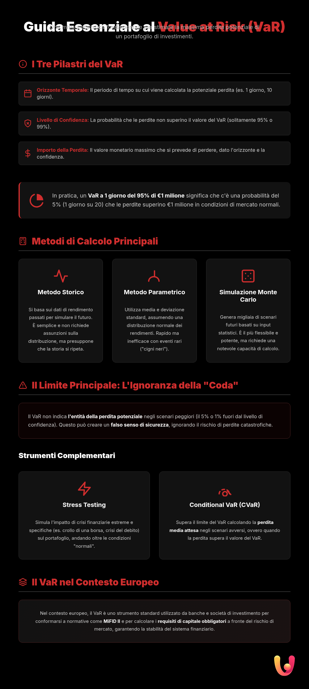
Value at Risk (VaR) is a statistical measure that quantifies the level of financial risk of an investment or portfolio. In simple terms, VaR answers a specific question: “What is the maximum loss I can reasonably expect to suffer over a given time frame, with a certain level of probability?”. To fully understand this definition, it’s essential to break it down into its three key elements: the time horizon, the confidence level, and the potential loss amount.
The time horizon is the reference period for the estimate, which can be a day, a week, or a month. The confidence level, usually set at 95% or 99%, indicates the probability that losses will not exceed the calculated value. Finally, the VaR itself is the maximum loss amount, expressed in absolute terms (e.g., $10,000) or as a percentage (e.g., 5% of the portfolio).
A one-day VaR of $5,000 with a 95% confidence level means there is a 95% probability that your portfolio will not lose more than $5,000 within the next day. Consequently, there is a 5% chance that the loss could be greater than that amount.
How is VaR Calculated? The Main Methods

There is no single formula for calculating VaR; its estimate can vary depending on the methodology used. Each approach has its own assumptions, advantages, and disadvantages, but all aim to provide a numerical summary of market risk. The three most common methods are the historical method, the parametric method, and the Monte Carlo simulation. The choice of method depends on the type of financial instruments in the portfolio, data availability, and the required level of accuracy.
The Historical Method
The historical simulation method is the most intuitive. It works on the assumption that the future will resemble the past. To calculate VaR, historical data of a portfolio’s daily returns are collected over a specific period (for example, the last two years). These returns are then sorted from worst to best. If a 95% confidence level is desired, you would identify the worst 5% of returns. The VaR will correspond to the minimum loss recorded in this range. Its strength is its simplicity, as it makes no assumptions about the statistical distribution of returns. However, its major limitation is that it relies entirely on past data, which may not be representative of future conditions, especially during periods of high turmoil.
The Parametric Method
The parametric approach, also known as the variance-covariance method, was popularized by J.P. Morgan in the 1990s. This method assumes that investment returns follow a normal distribution, the classic bell curve (Gaussian). To calculate VaR, two statistical parameters are needed: the mean return (the expected value) and the standard deviation, a measure of volatility. Although it is quick and easy to calculate, its main drawback lies in the assumption of normality. Financial markets are, in fact, known for their “black swans”—rare and extreme events that the normal curve fails to adequately predict.
The Monte Carlo Simulation
The Monte Carlo simulation is the most complex and flexible methodology. Unlike the other two approaches, it doesn’t just observe the past or make restrictive assumptions. Instead, it uses mathematical models to generate hundreds or thousands of possible future scenarios for the portfolio’s returns. For each scenario, the profit or loss is calculated. At the end of the simulation, a complete distribution of possible outcomes is obtained, from which the VaR for the desired confidence level can be derived. This method is very powerful because it can model even complex portfolios, but it requires significant computing power. If you want to learn more, you can read our guide on the Monte Carlo simulation for predicting uncertainty.
VaR in Practice: An Example for Better Understanding
To make the concept more concrete, let’s imagine an investor, Marco, who lives in Italy and has a portfolio of €100,000 invested in European market stocks. Concerned about market fluctuations, he asks his advisor to calculate the risk. The advisor analyzes the portfolio and tells Marco that “the 10-day VaR is €4,000, with a 99% confidence level“.
What does this sentence mean exactly? It means that, based on the statistical models used, there is a 99% probability that Marco’s portfolio will not lose more than €4,000 (4% of the total value) over the next 10 trading days. However, there is a small probability, 1%, that losses could exceed this threshold due to particularly adverse market events. Thanks to this single figure, Marco now has a quantitative idea of the risk he is taking, which is much more useful information than the generic statement “your portfolio has medium-to-high risk”.
VaR in the Italian and European Context: Between Tradition and Innovation
The application of risk management models like VaR takes on particular nuances when placed in the Italian and European context, where financial culture is a blend of tradition and a drive for innovation. The average Italian investor often shows a strong risk aversion, with a historical preference for tangible assets like “il mattone” (real estate) and instruments considered safe, such as government bonds. In this scenario, VaR acts as a bridge: it translates traditional prudence into a modern, quantifiable financial language, allowing for more conscious management of even the construction of a modern portfolio.
At the European level, regulations push for greater transparency and standardization. Regulations like MiFID II and directives from the European Banking Authority (EBA) and ESMA have made risk management a fundamental pillar for banks and investment firms. VaR has become a standard tool throughout the European Union for measuring market risk and for calculating the capital requirements that institutions must hold against their exposures. In this sense, VaR is not just a technical tool, but also a key element of quantitative analysis, promoting a common language of risk across the single financial market.
Limitations and Criticisms of Value at Risk
Despite its widespread use, VaR is not a perfect tool and has faced several criticisms, particularly after the 2008 financial crisis. Its main limitation is that it answers the question “what is my maximum probable loss?” but says nothing about the magnitude of the losses if one of those rare events that fall outside the confidence level occurs. In other words, a 99% VaR tells you that on only one day out of a hundred you might lose more than the indicated amount, but it doesn’t tell you if that loss will be slightly higher or catastrophic.
As the famous essayist Nassim Nicholas Taleb has pointed out, VaR can create a false sense of security by ignoring the potential impact of “black swans”—unpredictable events with devastating consequences.
To overcome this limitation, financial analysts often use VaR alongside other measures, such as Stress Testing (which simulates the impact of extreme crises) and Conditional VaR (CVaR) or Expected Shortfall. This latter indicator answers a more prudent question: “If things go wrong and I exceed the VaR threshold, what will be my average expected loss?”. The combined use of these tools offers a much more complete and robust view of risk.
In Brief (TL;DR)
Value at Risk (VaR) is a fundamental statistical indicator that helps you measure and manage the risk of your investments by estimating the maximum potential loss over a given time horizon.
Discover how this indicator measures the maximum potential loss of an investment portfolio within a specific time horizon and with a given confidence level.
Delve into the most common calculation methods, such as the historical and parametric methods, to apply this indicator to your portfolio management.
Conclusions

Value at Risk is not a crystal ball capable of predicting future losses with certainty, but rather a sophisticated ruler for measuring risk. Its greatest merit is its ability to summarize the market risk of an entire portfolio into a single number, making a complex concept easily understandable even for non-experts. It provides a fundamental reference point for making more informed and conscious investment decisions.
For the Italian investor and saver, understanding what VaR is means acquiring an additional tool for dialogue with their bank or financial advisor. It means moving from a generic perception of risk to its quantitative measurement. Although it is important to be aware of its limitations, VaR remains a pillar of modern risk management. Knowing it is the first step to navigating financial markets with greater confidence, protecting your savings, and building a more solid financial future.
Frequently Asked Questions

Value at Risk, or VaR, is a statistical measure that estimates the maximum potential loss an investment or portfolio could suffer over a specific period, with a certain level of probability. For example, a daily VaR of $1,000 at 95% confidence means there is a 95% probability that losses will not exceed $1,000 over the next day.
Even for a small investor, VaR is useful because it translates a complex concept like market risk into a single, easy-to-interpret number. It helps to become aware of the maximum potential loss under normal conditions, allowing one to choose investments more in line with their risk tolerance and to better diversify their portfolio.
There are three main methods. The ‘historical method’ is based on past returns to predict future losses. The ‘parametric method’ (or variance-covariance) uses statistical estimates like mean and standard deviation, assuming a normal distribution of returns. Finally, the ‘Monte Carlo simulation’ generates thousands of possible future scenarios to calculate risk, making it the most flexible but also the most complex.
No, VaR is not infallible and has significant limitations. Its main weakness is that it provides no information about the magnitude of losses that could occur in extreme scenarios, the so-called ‘black swans’—those events that fall outside the statistical confidence level (for example, in the 5% of cases not covered by a 95% VaR). For this reason, it is advisable to use it in conjunction with other risk metrics.
In Italy and Europe, VaR is a standard tool for banks and asset management companies. It is used for internal portfolio risk management and to comply with regulatory requirements imposed by authorities like the Bank of Italy and ESMA, within the framework of the Basel III accords. These regulations require banks to hold sufficient capital to cover potential losses, and VaR is one of the key tools for calculating this requirement.
Still have doubts about VaR: Calculate Risk and Protect Your Investments?
Type your specific question here to instantly find the official reply from Google.


Did you find this article helpful? Is there another topic you’d like to see me cover?
Write it in the comments below! I take inspiration directly from your suggestions.