Kalman Filter: Technical Guide for Finance and Lead Scoring

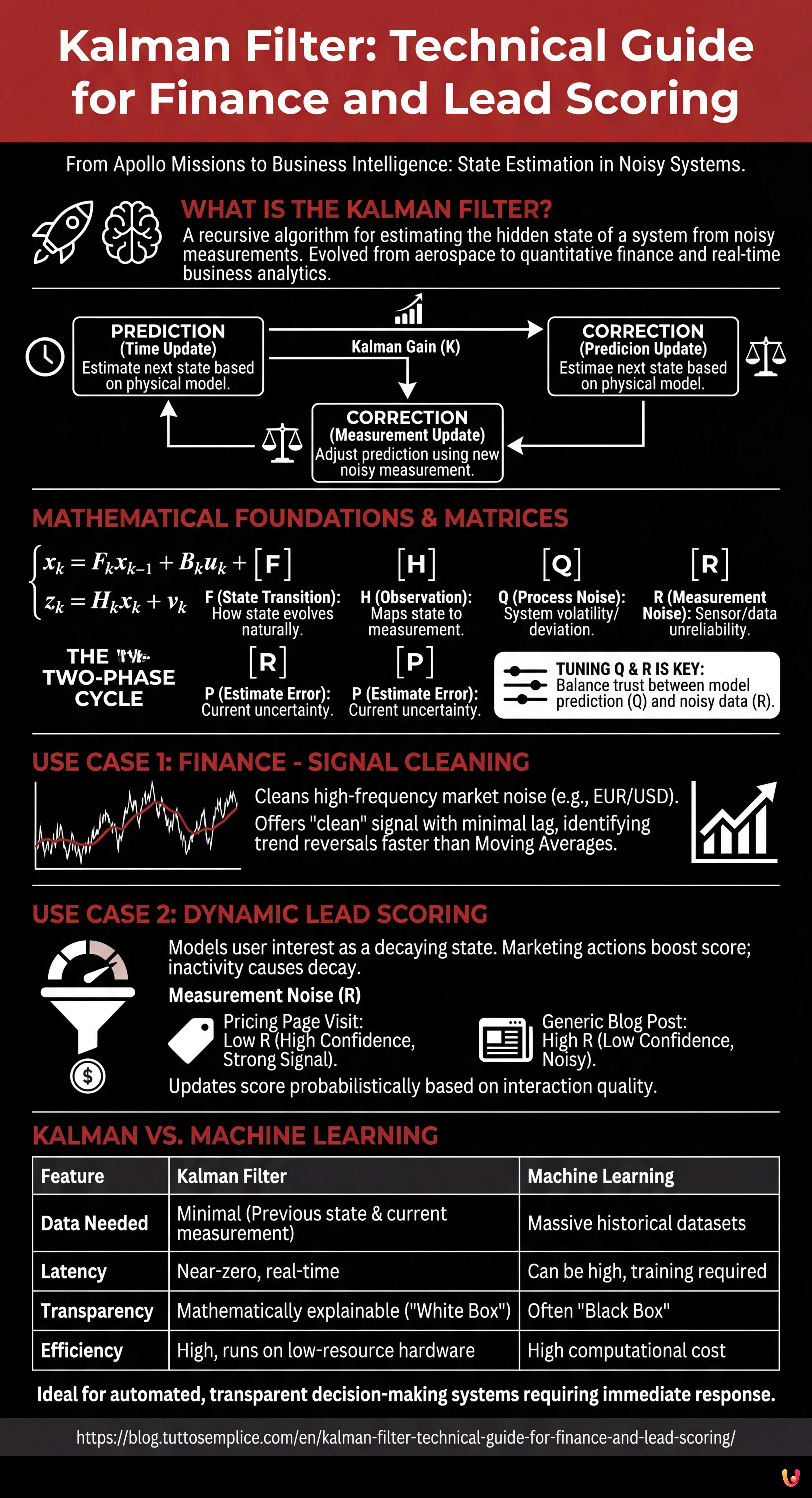
The Kalman filter is one of the cornerstones of control theory and systems engineering. Originally developed by Rudolf E. Kalman in 1960 and made famous by its use in the guidance computer of the Apollo missions, this recursive algorithm is the de facto standard for state estimation in noisy systems, from GPS navigation to robotics. However, in 2026, its application has transcended hardware to make a strong entry into the world of business intelligence and quantitative finance.

In this technical article, we will abandon superficial metaphors to focus on pure engineering applied to business data. We will see how to configure a Kalman filter for two critical purposes: signal cleaning in interest rate trends (removing high-frequency market noise) and dynamic estimation of lead quality (Lead Scoring) in real-time. Unlike “black box” Machine Learning models, the Kalman filter offers mathematical transparency and near-zero latency, making it ideal for automated decision-making systems.

Theoretical Foundations: Why the Kalman Filter?

The fundamental problem the filter solves is estimating the hidden state of a system ($x$) based on observable measurements ($z$) that are affected by noise. In a business context:

• The State ($x$): This is the “truth” we want to know. Example: a customer’s true interest (Lead Score) or the structural trend of an exchange rate.
• The Measurement ($z$): This is what we see. Example: a click on an email (which could be accidental) or the daily closing price (affected by speculative volatility).

The filter operates in a two-phase cycle: Prediction (Time Update) and Correction (Measurement Update). Its power lies in the ability to weigh the reliability of our mathematical prediction against the reliability of the new measurement, through a dynamically calculated variable called the Kalman Gain ($K$).

Mathematical Configuration of Matrices

To implement the filter, we must define the state equations. Let’s assume a discrete linear system:

$$x_k = F_k x_{k-1} + B_k u_k + w_k$$

$$z_k = H_k x_k + v_k$$

Where:

• $F$ (State Transition Matrix): How the state evolves on its own over time.
• $H$ (Observation Matrix): How the state is mapped into the measurement.
• $Q$ (Process Noise Covariance): How much the real system deviates from the ideal model ($w_k$).
• $R$ (Measurement Noise Covariance): How unreliable our sensors/data are ($v_k$).
• $P$ (Estimate Error Covariance): Our current uncertainty about the state estimation.

The Secret is in Q and R

The engineering “magic” lies in the tuning of $Q$ and $R$. If we set a high $R$, we tell the filter: “Don’t trust the measurements too much, they are noisy; trust the historical prediction more”. If we set a high $Q$, we say: “The system is very volatile, it changes direction rapidly”.

Use Case 1: Interest Rate Prediction and Cleaning

Financial markets are noisy. A Moving Average introduces an unacceptable lag for high-frequency trading. The Kalman filter, on the other hand, estimates the current state by minimizing the mean squared error, offering a “clean” signal with minimal delay.

Model Configuration

Let’s imagine tracking the EUR/USD. We consider state $x$ as a pair [Price, Velocity].

• Matrix $F$: Models the physics of the price. If we assume constant velocity:
  $$F = begin{bmatrix} 1 & Delta t 0 & 1 end{bmatrix}$$
• Matrix $H$: We only observe the price, not the velocity directly.
  $$H = begin{bmatrix} 1 & 0 end{bmatrix}$$
• Matrix $R$: Calculated based on the historical variance of intraday noise.

Applying this filter, we obtain a curve that ignores speculative spikes (noise $v_k$) but reacts promptly to structural trend changes (system dynamics), allowing the identification of market reversals sooner than an Exponential Moving Average (EMA).

Use Case 2: Dynamic Lead Scoring in the Funnel

In B2B marketing, traditional Lead Scoring is static (e.g., “Downloaded ebook = +5 points”). This approach ignores the decay of interest over time and the uncertainty of user actions. We can model a user’s interest as a physical state moving through space.

Modeling User Intent

We define state $x$ as a continuous scalar value from 0 to 100 (Interest Level).

1. Process Dynamics ($F$): Interest naturally decays over time if not nurtured. We can set $F = 0.95$ (daily exponential decay).
2. Control Input ($B cdot u$): Marketing actions (e.g., sending an email) are external forces that push the state upward.
3. Measurements ($z$): User interactions (clicks, site visits).
4. Measurement Noise ($R$): Here lies the genius. Not all clicks are equal.
   • Click on “Pricing Page”: Low $R$ (high confidence, strong signal).
   • Click on “Generic Blog Post”: High $R$ (low confidence, lots of noise).

The filter will update the lead score probabilistically. If a user visits the pricing page (strong measurement), the filter will drastically raise the estimate and reduce the covariance matrix $P$ (higher certainty). If the user disappears for two weeks, the dynamics $F$ will cause the score to decay, and $P$ will increase (we are less sure of their state).

Practical Implementation in Python

Here is a simplified example using the numpy library to implement a one-dimensional filter for Lead Scoring.

import numpy as np

class KalmanFilter:
    def __init__(self, F, B, H, Q, R, P, x):
        self.F = F  # State transition
        self.B = B  # Control matrix
        self.H = H  # Observation matrix
        self.Q = Q  # Process noise
        self.R = R  # Measurement noise
        self.P = P  # Error covariance
        self.x = x  # Initial state

    def predict(self, u=0):
        # State prediction
        self.x = self.F * self.x + self.B * u
        # Covariance prediction
        self.P = self.F * self.P * self.F + self.Q
        return self.x

    def update(self, z):
        # Measurement residual calculation
        y = z - self.H * self.x
        # Kalman Gain calculation (K)
        S = self.H * self.P * self.H + self.R
        K = self.P * self.H / S
        
        # State and covariance update
        self.x = self.x + K * y
        self.P = (1 - K * self.H) * self.P
        return self.x

# Configuration for Lead Scoring
# Initial state: 50/100, High uncertainty P
kf = KalmanFilter(F=0.98, B=5, H=1, Q=0.1, R=10, P=100, x=50)

# Day 1: No action (Decay)
print(f"Day 1 (No actions): {kf.predict(u=0):.2f}")

# Day 2: User visits Pricing (Measurement z=90, dynamic low R)
kf.R = 2 # High confidence
kf.predict(u=0)
print(f"Day 2 (Pricing Visit): {kf.update(z=90):.2f}")

Kalman vs Machine Learning: Why choose the former?

In the era of Generative AI and deep neural networks, why go back to an algorithm from 1960? The answer lies in efficiency and explainability.

• Data required: Neural networks require terabytes of historical data for training. The Kalman filter requires only the previous state and the current measurement. It is operational from “Day 1”.
• Computational Cost: The Kalman filter consists of simple matrix operations. It can run on microcontrollers or overloaded servers with negligible latency.
• Transparency: If the model makes a mistake, we can inspect matrix $P$ or gain $K$ to understand exactly why. It is not a “Black Box”.

Conclusions

Applying the Kalman filter outside of electronic engineering requires a paradigm shift: one must stop viewing business data as simple numbers and start viewing them as signals emitted by a dynamic system. Whether predicting the trajectory of a missile or a customer’s propensity to buy, the mathematics of state estimation remains the same. For companies seeking real-time competitive advantages, mastering these control tools offers a clear strategic edge over competitors who still rely on static averages or opaque and slow ML models.

Frequently Asked Questions

Sources and Further Reading

1. General Overview and Mathematical Definition of the Kalman Filter – Wikipedia
2. Discovery of the Kalman Filter as a Practical Tool for Aerospace – NASA Technical Reports Server
3. Application of Kalman Filtering in Estimating Interest Rates – Federal Reserve Bank of New York
4. National Medal of Science Awarded to Rudolf E. Kalman – National Science Foundation

Francesco Zinghinì

Electronic Engineer with a mission to simplify digital tech. Thanks to his background in Systems Theory, he analyzes software, hardware, and network infrastructures to offer practical guides on IT and telecommunications. Transforming technological complexity into accessible solutions.

LinkedInFacebookFull Bio →