Time Series Analysis: Signal Processing for Business KPIs

In the landscape of modern Business Intelligence, time series analysis often represents the boundary between a decision based on intuition and one founded on data science. However, most analysts limit themselves to observing moving averages and percentage variations, ignoring a methodological heritage that electronic engineering has perfected over the last few decades: Signal Processing (Digital Signal Processing).

In this technical guide, we will abandon the classic statistical approach to adopt an engineering vision. We will treat business KPIs (such as the volume of mortgage requests in a Fintech or daily cash flow) not as simple numbers on a spreadsheet, but as electrical signals affected by noise. By applying mathematical transforms and digital filters, we will learn to extract the “pure trend” (the signal) from random market fluctuations (the noise).

1. The Engineering Mindset: Signal vs Noise

In electronics, a signal received by a sensor is always contaminated by external disturbances. The same happens in business data. If we look at the graph of daily sales, we see peaks and valleys. The fundamental question is: is that dip on Tuesday a worrying trend (Signal) or just a random variation due to weather or a public holiday (Noise)?

To answer, we must define the SNR – Signal-to-Noise Ratio. An approach based on system physics teaches us that:

• The Signal is deterministic information, often low frequency (growth trend) or with specific frequency (seasonality).
• The Noise is stochastic, often high frequency and randomly distributed (Gaussian white noise).

2. Tools and Prerequisites

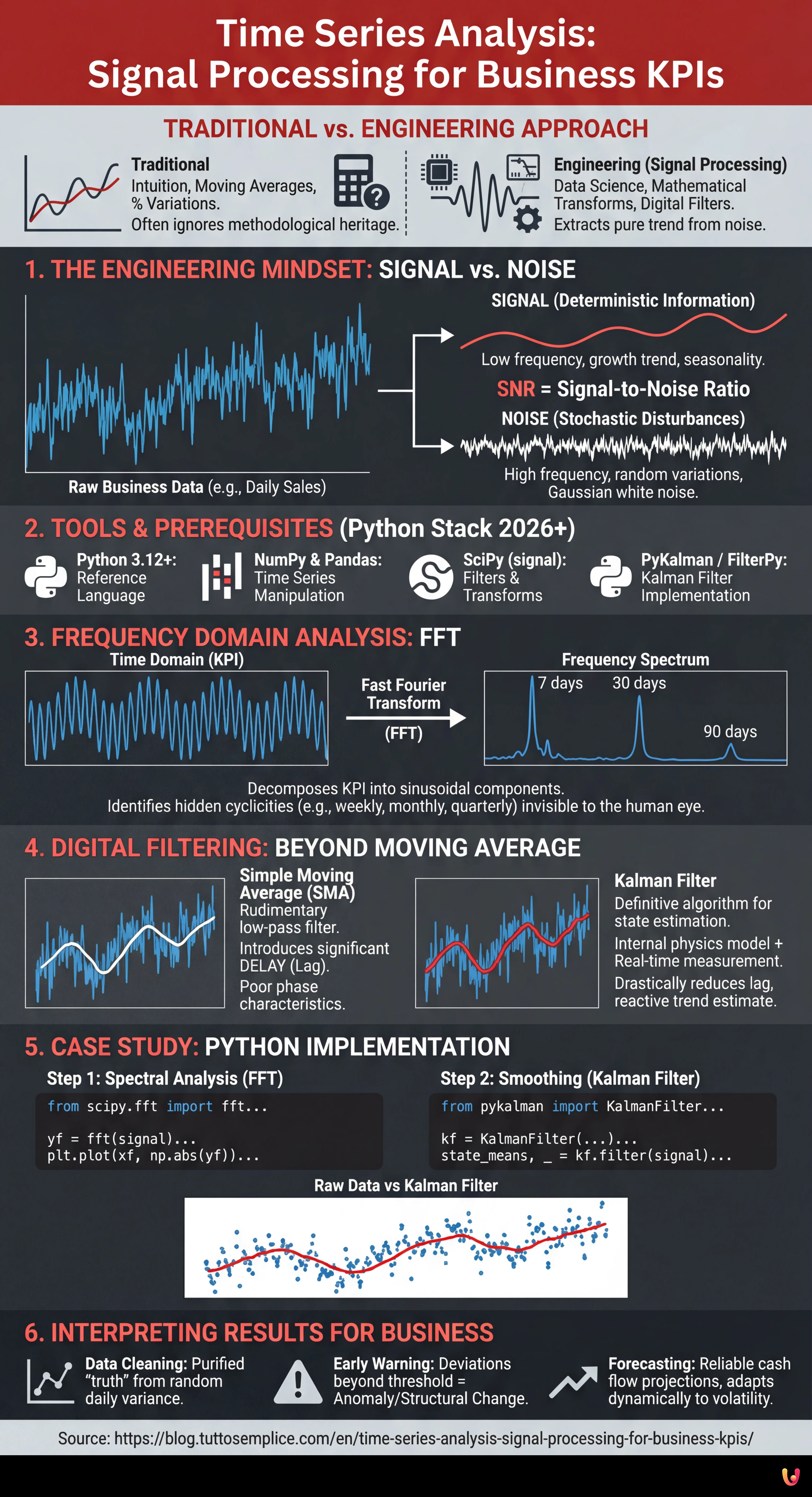
To follow this guide, we will not use Excel. Advanced signal analysis requires computing power and specific libraries. As of 2026, the standard stack for this type of operation includes:

• Python 3.12+: The reference language.
• NumPy & Pandas: For time series manipulation.
• SciPy (module signal): For implementing digital filters and transforms.
• PyKalman or FilterPy: Libraries optimized for Kalman filter implementation.

3. Frequency Domain Analysis: The Fourier Transform (FFT)

One of the most common mistakes in financial time series analysis is trying to intuit seasonality by looking at the graph in the time domain. An electronic engineer, however, moves the problem into the frequency domain.

Using the Fast Fourier Transform (FFT), we can decompose our KPI (e.g., daily mortgage requests) into its constituent sinusoidal components. This allows us to identify hidden cyclicities that the human eye cannot see.

Practical Application: Detecting Mortgage Cyclicity

Imagine having a dataset of 365 days of requests. By applying the FFT, we might see a magnitude peak at the frequency corresponding to 7 days (weekly cycle) and one at 30 days (monthly cycle). If we notice an unexpected peak at 90 days, we have discovered a quarterly cyclicity linked, for example, to tax deadlines, without having to guess it.

4. Digital Filtering: Beyond the Moving Average

Once we understand the spectrum of our signal, we must clean it. The technique most used in business is the Simple Moving Average (SMA). In engineering, the SMA is considered a very rudimentary low-pass filter with poor phase characteristics (it introduces significant delay, or lag).

The Lag Problem

If you use a 30-day moving average to forecast cash flow, your indicator will tell you that the trend changed with a 15-day delay. In a volatile market like Fintech, this delay is unacceptable.

The Solution: The Kalman Filter

The Kalman Filter is the definitive algorithm for state estimation in dynamic systems (used from GPS to missile guidance systems). Unlike moving averages, the Kalman filter does not limit itself to “smoothing” the past, but:

1. Possesses an internal model of the system physics (e.g., the expected growth trend).
2. Compares the model prediction with the new real measurement (today’s data).
3. Calculates the Kalman Gain: decides how much to trust the model and how much to trust the new measurement based on the uncertainty (covariance) of both.

The result is an extremely reactive trend estimate that separates noise from the real signal almost in real-time, drastically reducing lag.

5. Case Study: Implementation in Python

Let’s see how to apply these concepts to a fictitious dataset of daily loan requests.

Step 1: Spectral Analysis with FFT

import numpy as np
import pandas as pd
from scipy.fft import fft, fftfreq
import matplotlib.pyplot as plt

# Load data (Time Series)
data = pd.read_csv('mortgage_requests.csv')
signal = data['requests'].values

# Calculate FFT
N = len(signal)
T = 1.0 / 365.0 # Daily sampling
yf = fft(signal)
xf = fftfreq(N, T)[:N//2]

# Plot spectrum
plt.plot(xf, 2.0/N * np.abs(yf[0:N//2]))
plt.title('Frequency Spectrum (Cyclicity)')
plt.grid()
plt.show()

Interpretation: The peaks in the graph indicate the natural cycles of the business. If we eliminate these frequencies (notch filter), we obtain the seasonally adjusted trend in a mathematically rigorous way.

Step 2: Smoothing with Kalman Filter

To clean the signal while maintaining reactivity, we use a basic implementation of a one-dimensional Kalman filter.

from pykalman import KalmanFilter

# Filter Configuration
# transition_covariance: how fast the real trend changes
# observation_covariance: how much noise is in the daily data
kf = KalmanFilter(transition_matrices=[1],
                  observation_matrices=[1],
                  initial_state_mean=signal[0],
                  initial_state_covariance=1,
                  observation_covariance=10,
                  transition_covariance=0.1)

# Calculate filtered signal
state_means, _ = kf.filter(signal)

# Comparison
data['Kalman_Signal'] = state_means
data[['requests', 'Kalman_Signal']].plot()
plt.title('Raw Data vs Kalman Filter')
plt.show()

6. Interpreting Results for Business

Applying these time series analysis techniques transforms the decision-making process:

• Data Cleaning: The line generated by the Kalman filter (state_means) represents the business “truth”, purified from random daily variance.
• Early Warning: If the real data deviates from the Kalman filter beyond a certain threshold (e.g., 3 standard deviations of the residual covariance), it is not noise: it is an anomaly or a structural market change requiring immediate intervention.
• Forecasting: By projecting the Kalman filter state into the future, we obtain cash flow forecasts that are much more reliable than linear regression, because the filter adapts dynamically to the speed of system change.

Conclusions

Treating business data as electrical signals is not just an academic exercise, but a competitive advantage. While competitors react to noise (e.g., a day of poor sales due to chance), the company using Signal Processing stays the course, reacting only when the signal indicates a real structural change. The use of the Fourier Transform and the Kalman Filter elevates time series analysis from simple observation to a high-precision predictive tool.

Frequently Asked Questions

Francesco Zinghinì

Electronic Engineer with a mission to simplify digital tech. Thanks to his background in Systems Theory, he analyzes software, hardware, and network infrastructures to offer practical guides on IT and telecommunications. Transforming technological complexity into accessible solutions.

LinkedInFacebookFull Bio →